HW 3 DC Circuit Solver

In this project, you will implement a basic DC circuit solver. The solving engine will be built on a basic matrix linear algebra library using a multiply-linked list to represent a sparse matrix. The circuit description and simulation commands will be read from a file.

• HW 3 DC Circuit Solver
• Input File Format
  • Resistance
  • Voltage Source
  • Print Node
  • Example Input File
• Command line
• How to compute a DC solution:
• Design Limitations and Details
• Functions required (TAs may look for, inspect, and grade these, points may be deducted for those missing)
• How to compute row reduced echelon form:
• Examples
  • Example 1 Resistor Divider
    • Equations
    • All together
    • Matrix Form
    • Row Operations
    • Example with augmented matrix as your program will generate and operate on numerically
      • Row Combine
      • Row-Scaling
      • Backward Row Combine
  • Example 2
    • Operation-by-Operation Example on Augmented Matrix
    • Operation-by-Operation Example on Augmented Matrix, Requiring initial row-swap
    • Deriving the augmented matrix manually
    • Working with the augmented matrix symbolically

Input File Format

Syntax	Description
<name>	name formed by ASCII characters ‘0’-‘9’,‘a’-‘z’,‘A-Z’,’_’
<ws>	any sequence of whitespace characters
<nn1>,<nn2>	integer specified using ASCII characters ‘0’-‘9’
<value>	floating point value specified using characters ‘0’-‘9’,’.’,‘e’,‘E,’+’,’-’
<NL>	UNIX newline

Resistance

R<name><ws><nn1><ws><nn2><ws><value><NL>

You may ignore any devices whose terminals are shorted (i.e. ignore device if nn1==nn2)

Voltage Source

V<alphanumname><ws><nn1><ws><value><NL>

Voltage source may only exist from ground to a node. You may assume no two voltage sources are connected to the same node.

Print Node

P<ws><nn1><NL>

These designate which node results should be printed.

Example Input File

R1 1 2 2
R2 1 3 4
R3 2 3 5.2
R4 3 4 6
R5 2 4 3
V1 1 6
V2 4 2
P 1

Command line

The name of your program should be cs and should be called with the input file as an argument.

cs <filename>

Example:

cs circuit.cs

How to compute a DC solution:

Assume $A$ is initially a zero matrix of size $n\times n$ where $n$ is the number of nodes. Assume $b$ is $n\times1$.

For each component connected between some i and j (if the component’s terminals are shorted, i=j, you may ignore it)

• Add $-1/R_{ij}$ to $A_{ij}$ and $A_{ji}$

• Add $1/R_{ij}$ to $A_{ii}$ and $A_{jj}$

Then, for each source node node i.

• Set row $i$ in $A$ to all zeros, then set $A_{ii}=1$

• set $b_{i} = \rm voltage$

To solve the circuit,

• Let $G=A|b;$
  • G is an augmented matrix
• Let $F=\rm rref(G);$
  • row reduced echelon form
• Let $s=\text{last column of }F;$
  • s is the solution, one voltage for each node

Design Limitations and Details

• Terms are implemented with a minmum of these 7 elements of information:

• value is a float

• row,col are integers

• up,down,left,right are pointers to the next non-zero term in each direction or NULL pointers if non exists

• A given matrix is implemented as a multiply-linked list such that each term is part of two linked list, one row-wise and one column-wise.

• Implement Base ADT functions first. You must write functions to create and destroy stand-alone nodes, insert and delete nodes from a linked list, and mutators to modify node data or pointers, deallocation of all nodes in a list, deep copy and shallow copy of a list. I strongly recommend these as well: print node, print column,print row, print matrix.

• A note on invalid input files: If an input file is invalid, your program behavior may be undefined and this is excused, except that invalid memory access/segmentation faults is not excused

• global variables are not allowed on this project

• Report guidelines will be posted at a later time.

• Example files will be posted, though it is not guaranteed that they are comprehensive tests.

Functions required (TAs may look for, inspect, and grade these, points may be deducted for those missing)

• AddToElementValue(A,r,c,s) modifies matrix $A$, adding scalar to element: $A_{r,c}=A_{r,c}+s$

• SetElementValue(A,r,c,s) modifies matrix $A$, sets $A_{r,c}=s$. Should remove and destroy element if s=0

• GetElementValue(A,r,c) returns value $A_{r,c}$

• FindLargestInCol(A,c) returns pointer to term with largest value (maximum absolute value)

• RowSwap(A,r1,r2) modifies A by performing a row swap

• ScaleRow(A,r,s) modifies A by multiplying row r by scalar s

• RowCombine(A,r1,r2,s) modifies row r1 of A by adding row r2 scaled by scalar s

• AugmentMatrix(A,B) augments B to right of A, modifying A and emptying B in the process (moves nodes from B to A appropriately)

• CopySubMatrix(A,B,rowStart,rowEnd,columnStart,columnEnd) deep copies submatrix of B to an empty A, if A is not empty then A is first emptied

How to compute row reduced echelon form:

PSEUDO CODE

//computes same as u in Matlab: [~,u]=lu(A);
for colItr 1 to m,
  //find value largest possible pivot value in column
  largestNodePtr = FindMaxAbsInCol(list,col#);
  //if largest value is zero matrix is singular
  if (GetElementValue(largestNodePtr)) == 0,           
        error('Matrix is Singular');

  //swap current row with lagest pivot value row
  RowSwap(A,colItr,GetRowIndex(largestColumnNodePtr)); 

 //create zeros below pivot point
  for itrR = (colItr +1) to m,                         
        RowCombine(itrR,colItr,
            -1*GetElementValue(A,itrR,colItr)
            /GetElementValue(A,colItr,colItr));
  end
end

//now finish computing rref(A)
//make all pivots points ones by dividing each row by the pivot value
//  then reduce matrix by creating zeros above pivot points
for diagonalItr = 1:n
  ScaleRow(A,diagonalItr, 1/GetElementValue(A,diagonalItr,diagonalItr)); 
  for rowItr =1 1 to (colItr-1)
    RowCombine(A, rowItr,diagonalItr, -(A(rowItr,diagonalItr));
  end
end

Examples

Example 1 Resistor Divider

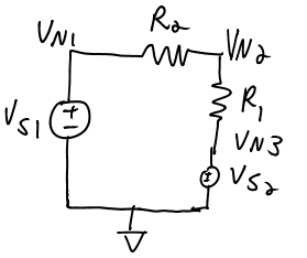
• Write 3 equations for 3 variables (in this case two are known immediately by noticing the voltage components).
• Let the nodes voltages be $V_{N1}$,$V_{N2}$,and $V_{N3}$

Let the voltage source be $V_{S1}$ and $V_{S2}$

Equations

Eqn1@Node1:

• $V_{N1}=V_{S1}$

Eqn2@Node2:

• Current Out due to voltage VN2 = Current In due to surrounding voltages
• $\frac{V_{N1}-V_{N2}}{R_{2}}=\frac{V_{N2}-V_{N3}}{R_{1}}$
• $V_{N1}\left(\frac{1}{R_{2}}\right)+V_{N3}\left(\frac{1}{R1}\right)=V_{N2}\left(\frac{1}{R_{1}}+\frac{1}{R2}\right)$
• $0=V_{N1}\left(\frac{1}{R_{2}}\right)-V_{N2}\left(\frac{1}{R_{1}}+\frac{1}{R_{2}}\right)+V_{N3}\left(\frac{1}{R_{1}}\right)\leftarrow$ use this one

Eqn3@Node3:

• $V_{N3}=V_{S2}$

All together

$\begin{array}{cccc} V_{S1}= & V_{N1}\times1 & +V_{N2}\times0 & +V_{N3}\times0\\ 0= & V_{N1}\times\left(1/R_{2}\right) & -V_{N2}\times\left(1/R_{1}+1/R_{2}\right) & +V_{N3}\times\left(1/R_{1}\right)\\ V_{S2}= & V_{N1}\times0 & +V_{n2}\times0 & +V_{N3}\times1 \end{array}$

Matrix Form

In matrix form, we write this as

$\underbrace{\left[\begin{array}{c} V_{S1}\\ 0\\ V_{S2} \end{array}\right]}_{b}=\underbrace{\left[\begin{array}{ccc} 1 & 0 & 0\\ \left(1/R_{1}\right) & -\left(1/R_{1}+1/R_{2}\right) & \left(1/R_{1}\right)\\ 0 & 0 & 1 \end{array}\right]}_{A}\underbrace{\left[\begin{array}{c} V_{N1}\\ V_{N2}\\ V_{N3} \end{array}\right]}_{x}$

$b=Ax$

Look at how the order of of the equations is represented in the matrix and can be reordered:

Likewise, we can combine and manipulate rows in the matrix just corresponding to manipulations of the original equations, but in a compact written form.

Such simple row operations operations can be used to solve for x as follows.

• $x=b/A$
• $x=A^{-1}b$

Manipulating the equations can accomplish the matrix inversion $A \rightarrow A^{-1}$. As it turns out, performing the same manipulations on $b$ that make $A$ into an identity matrix provides the solution for $x$ in terms of all provided values. To make this easier, we write $A$ next to $b$ as one matrix and call it the augmented matrix, $A|b$.

Row Operations

Row2 = Row2 + Row1 $\times-\frac{1}{R_{2}}$

$\left[\begin{array}{c} V_{S1}\\ -\frac{1}{R_{2}}V_{S1}\\ V_{S2} \end{array}\right]=\left[\begin{array}{ccc} \textcircled{1} & 0 & 0\\ \boxed{0} & -\left(1/R_{1}+1/R_{2}\right) & \left(1/R_{1}\right)\\ 0 & 0 & 1 \end{array}\right] \left[\begin{array}{c} V_{N1}\\ V_{N2}\\ V_{N3} \end{array}\right]$

Row2 = Row2 $\times\frac{1}{\frac{1}{R_{1}}+\frac{1}{R_{2}}}$

$\left[\begin{array}{c} V_{S1}\\ \frac{-\frac{1}{R_{2}}}{-\left(1/R_{1}+1/R_{2}\right)}V_{S1}\\ V_{S2} \end{array}\right]=\left[\begin{array}{ccc} 1 & 0 & 0\\ 0 & \textcircled{\boxed{1}} & \frac{\left(1/R_{1}\right)}{-\left(1/R_{1}+1/R_{2}\right)}\\ 0 & 0 & 1 \end{array}\right]\left[\begin{array}{c} V_{N1}\\ V_{N2}\\ V_{N3} \end{array}\right]$

Row2 = Row 2 + Row3 $\times\frac{\left(1/R_{1}\right)}{-\left(1/R_{1}+1/R_{2}\right)}$

$\left[\begin{array}{c} V_{S1}\\ \frac{-\frac{1}{R_{2}}V_{S1}-\frac{1}{R_{1}}V_{S2}}{-\left(1/R_{1}+1/R_{2}\right)}\\ V_{S2} \end{array}\right]=\left[\begin{array}{ccc} 1 & 0 & 0\\ 0 & 1 & \boxed{0}\\ 0 & 0 & \textcircled{1} \end{array}\right]\left[\begin{array}{c} V_{N1}\\ V_{N2}\\ V_{N3} \end{array}\right]$

Now, with just simplification of expressions…
(only for symbolic computation, in your numerical solver this step would not exist)

$\left[\begin{array}{c} V_{S1}\\ \frac{R_{1}V_{S1}+R_{2}V_{S2}}{R_{1}+R_{2}}\\ V_{S2} \end{array}\right]=\left[\begin{array}{ccc} 1 & 0 & 0\\ 0 & 1 & 0\\ 0 & 0 & 1 \end{array}\right]\left[\begin{array}{c} V_{N1}\\ V_{N2}\\ V_{N3} \end{array}\right]$

$\left[\begin{array}{c} V_{S1}\\ \frac{R_{1}V_{S1}+R_{2}V_{S2}}{R_{1}+R_{2}}\\ V_{S2} \end{array}\right]=\left[\begin{array}{c} V_{N1}\\ V_{N2}\\ V_{N3} \end{array}\right]$

Example with augmented matrix as your program will generate and operate on numerically

Your program’s initial effort is to directly generate this matrix:
$\underbrace{\left[\begin{array}{ccc} 1 & 0 & 0 & V_{S1}\\ \left(1/R_{1}\right) & -\left(1/R_{1}+1/R_{2}\right) & \left(1/R_{1}\right) & 0\\ 0 & 0 & 1 & V_{S2} \end{array}\right]}_{A|b}$

Though it is shown symbolically here, you are provided numerical values and will perform numerical computation to make the A matrix an identity matrix (all-zeros except ones on the diagonal)

Row Combine

Using Row1 to eliminate the first-column element in Row2
Row2 = Row2 + Row1 $\times-\frac{1}{R_{2}}$

$\left[\begin{array}{ccc} \textcircled{1} & 0 & 0 & V_{S1}\\ \boxed{0} & -\left(1/R_{1}+1/R_{2}\right) & \left(1/R_{1}\right)& -\frac{1}{R_{2}}V_{S1}\\ 0 & 0 & 1 & V_{S2} \end{array}\right]$

Row-Scaling

Scaling Row2 so that the second-column element is 1
Row2 = Row2 $\times - \frac{1}{\frac{1}{R_{1}}+\frac{1}{R_{2}}}$

$\left[\begin{array}{ccc} 1 & 0 & 0 & V_{S1}\\ 0 & \textcircled{\boxed{1}} & \frac{\left(1/R_{1}\right)}{-\left(1/R_{1}+1/R_{2}\right)} & \frac{-\frac{1}{R_{2}}}{-\left(1/R_{1}+1/R_{2}\right)}V_{S1}\\ 0 & 0 & 1 & V_{S2} \end{array}\right]$

Backward Row Combine

Row2 = Row 2 + Row3 $\times\frac{\left(1/R_{1}\right)}{-\left(1/R_{1}+1/R_{2}\right)}$

$\left[\begin{array}{ccc} 1 & 0 & 0 & V_{S1}\\ 0 & 1 & \boxed{0} & \frac{-\frac{1}{R_{2}}V_{S1}-\frac{1}{R_{1}}V_{S2}}{-\left(1/R_{1}+1/R_{2}\right)}\\ 0 & 0 & \textcircled{1} & V_{S2} \end{array}\right]$

At this point in your program, the left matrix is an identity matrix the computation is done since it is numerical.

Example 2

See circuit at http://matlabbyexamples.blogspot.com/2011_11_01_archive.html

Example input file:

R1 1 2 2
R2 1 3 4
R3 2 3 5.2
R4 3 4 6
R5 2 4 3
VS1 1 6
VS2 4 0
P 1

Results by running the matlab code exactly as provided on the website.

>> A

A =

    1.0000         0         0         0
   -0.5000    1.0256   -0.1923   -0.3333
   -0.2500   -0.1923    0.6090   -0.1667
         0         0         0    1.0000

B =

     6
     0
     0
     2

Therefore the initial augmented matrix that you should generate is

    1.0000         0         0         0  6
   -0.5000    1.0256   -0.1923   -0.3333  0
   -0.2500   -0.1923    0.6090   -0.1667  0
         0         0         0    1.0000  2

Finally the provided matlab code produces the following result:

>>  Vo=A\B; 
disp(Vo); 
    6.0000
    4.4000
    4.4000
    2.0000

>> 

Operation-by-Operation Example on Augmented Matrix

    +1.000000  +0.000000  +0.000000  +0.000000  +6.000000  
    -0.500000  +1.025600  -0.192300  -0.333300  +0.000000  
    -0.250000  -0.192300  +0.609000  -0.166700  +0.000000  
    +0.000000  +0.000000  +0.000000  +1.000000  +2.000000  

*** Working on Coumn 1 ***
No intial row-swap Required for pivot column 1
Scale: Row1=1.0*Row1
    +1.000000  +0.000000  +0.000000  +0.000000  +6.000000  
    -0.500000  +1.025600  -0.192300  -0.333300  +0.000000  
    -0.250000  -0.192300  +0.609000  -0.166700  +0.000000  
    +0.000000  +0.000000  +0.000000  +1.000000  +2.000000  
Combine: Row2=Row2+0.5*Row1
    +1.000000  +0.000000  +0.000000  +0.000000  +6.000000  
    +0.000000  +1.025600  -0.192300  -0.333300  +3.000000  
    -0.250000  -0.192300  +0.609000  -0.166700  +0.000000  
    +0.000000  +0.000000  +0.000000  +1.000000  +2.000000  
Combine: Row3=Row3+0.25*Row1
    +1.000000  +0.000000  +0.000000  +0.000000  +6.000000  
    +0.000000  +1.025600  -0.192300  -0.333300  +3.000000  
    +0.000000  -0.192300  +0.609000  -0.166700  +1.500000  
    +0.000000  +0.000000  +0.000000  +1.000000  +2.000000  
Row4 pivot column is already 0

*** Working on Coumn 2 ***
No intial row-swap Required for pivot column 2
Scale: Row2=0.9750390015600623*Row2
    +1.000000  +0.000000  +0.000000  +0.000000  +6.000000  
    +0.000000  +1.000000  -0.187500  -0.324980  +2.925117  
    +0.000000  -0.192300  +0.609000  -0.166700  +1.500000  
    +0.000000  +0.000000  +0.000000  +1.000000  +2.000000  
Combine: Row3=Row3+0.1923*Row2
    +1.000000  +0.000000  +0.000000  +0.000000  +6.000000  
    +0.000000  +1.000000  -0.187500  -0.324980  +2.925117  
    +0.000000  +0.000000  +0.572944  -0.229194  +2.062500  
    +0.000000  +0.000000  +0.000000  +1.000000  +2.000000  
Row4 pivot column is already 0

*** Working on Coumn 3 ***
No intial row-swap Required for pivot column 3
Scale: Row3=1.745372036958253*Row3
    +1.000000  +0.000000  +0.000000  +0.000000  +6.000000  
    +0.000000  +1.000000  -0.187500  -0.324980  +2.925117  
    +0.000000  +0.000000  +1.000000  -0.400028  +3.599830  
    +0.000000  +0.000000  +0.000000  +1.000000  +2.000000  
Row4 pivot column is already 0
Scale: Row4=1.0*Row4
    +1.000000  +0.000000  +0.000000  +0.000000  +6.000000  
    +0.000000  +1.000000  -0.187500  -0.324980  +2.925117  
    +0.000000  +0.000000  +1.000000  -0.400028  +3.599830  
    +0.000000  +0.000000  +0.000000  +1.000000  +2.000000  

*** Working on Coumn 4 ***
Combine: Row3=Row3+0.40002836229560057*Row4
    +1.000000  +0.000000  +0.000000  +0.000000  +6.000000  
    +0.000000  +1.000000  -0.187500  -0.324980  +2.925117  
    +0.000000  +0.000000  +1.000000  +0.000000  +4.399887  
    +0.000000  +0.000000  +0.000000  +1.000000  +2.000000  
Combine: Row2=Row2+0.32498049921996874*Row4
    +1.000000  +0.000000  +0.000000  +0.000000  +6.000000  
    +0.000000  +1.000000  -0.187500  +0.000000  +3.575078  
    +0.000000  +0.000000  +1.000000  +0.000000  +4.399887  
    +0.000000  +0.000000  +0.000000  +1.000000  +2.000000  
Row1 pivot column is already 0

*** Working on Coumn 3 ***
Combine: Row2=Row2+0.18749999999999997*Row3
    +1.000000  +0.000000  +0.000000  +0.000000  +6.000000  
    +0.000000  +1.000000  +0.000000  +0.000000  +4.400057  
    +0.000000  +0.000000  +1.000000  +0.000000  +4.399887  
    +0.000000  +0.000000  +0.000000  +1.000000  +2.000000  
Row1 pivot column is already 0

*** Working on Coumn 2 ***
Row1 pivot column is already 0

Operation-by-Operation Example on Augmented Matrix, Requiring initial row-swap

Same as above, but with input Row2 and input Row3 swapped, requiring a swap when working on pivot column 2 to get the largest possible pivot-position value.

    +1.000000  +0.000000  +0.000000  +0.000000  +6.000000  
    -0.250000  -0.192300  +0.609000  -0.166700  +0.000000  
    -0.500000  +1.025600  -0.192300  -0.333300  +0.000000  
    +0.000000  +0.000000  +0.000000  +1.000000  +2.000000  

*** Working on Coumn 1 ***
No intial row-swap Required for pivot column 1
Scale: Row1=1.0*Row1
    +1.000000  +0.000000  +0.000000  +0.000000  +6.000000  
    -0.250000  -0.192300  +0.609000  -0.166700  +0.000000  
    -0.500000  +1.025600  -0.192300  -0.333300  +0.000000  
    +0.000000  +0.000000  +0.000000  +1.000000  +2.000000  
Combine: Row2=Row2+0.25*Row1
    +1.000000  +0.000000  +0.000000  +0.000000  +6.000000  
    +0.000000  -0.192300  +0.609000  -0.166700  +1.500000  
    -0.500000  +1.025600  -0.192300  -0.333300  +0.000000  
    +0.000000  +0.000000  +0.000000  +1.000000  +2.000000  
Combine: Row3=Row3+0.5*Row1
    +1.000000  +0.000000  +0.000000  +0.000000  +6.000000  
    +0.000000  -0.192300  +0.609000  -0.166700  +1.500000  
    +0.000000  +1.025600  -0.192300  -0.333300  +3.000000  
    +0.000000  +0.000000  +0.000000  +1.000000  +2.000000  
Row4 pivot column is already 0

*** Working on Coumn 2 ***
Swap: Row 3 into pivot row 2
    +1.000000  +0.000000  +0.000000  +0.000000  +6.000000  
    +0.000000  +1.025600  -0.192300  -0.333300  +3.000000  
    +0.000000  -0.192300  +0.609000  -0.166700  +1.500000  
    +0.000000  +0.000000  +0.000000  +1.000000  +2.000000  
Scale: Row2=0.9750390015600623*Row2
    +1.000000  +0.000000  +0.000000  +0.000000  +6.000000  
    +0.000000  +1.000000  -0.187500  -0.324980  +2.925117  
    +0.000000  -0.192300  +0.609000  -0.166700  +1.500000  
    +0.000000  +0.000000  +0.000000  +1.000000  +2.000000  
Combine: Row3=Row3+0.1923*Row2
    +1.000000  +0.000000  +0.000000  +0.000000  +6.000000  
    +0.000000  +1.000000  -0.187500  -0.324980  +2.925117  
    +0.000000  +0.000000  +0.572944  -0.229194  +2.062500  
    +0.000000  +0.000000  +0.000000  +1.000000  +2.000000  
Row4 pivot column is already 0

*** Working on Coumn 3 ***
No intial row-swap Required for pivot column 3
Scale: Row3=1.745372036958253*Row3
    +1.000000  +0.000000  +0.000000  +0.000000  +6.000000  
    +0.000000  +1.000000  -0.187500  -0.324980  +2.925117  
    +0.000000  +0.000000  +1.000000  -0.400028  +3.599830  
    +0.000000  +0.000000  +0.000000  +1.000000  +2.000000  
Row4 pivot column is already 0
Scale: Row4=1.0*Row4
    +1.000000  +0.000000  +0.000000  +0.000000  +6.000000  
    +0.000000  +1.000000  -0.187500  -0.324980  +2.925117  
    +0.000000  +0.000000  +1.000000  -0.400028  +3.599830  
    +0.000000  +0.000000  +0.000000  +1.000000  +2.000000  

*** Working on Coumn 4 ***
Combine: Row3=Row3+0.40002836229560057*Row4
    +1.000000  +0.000000  +0.000000  +0.000000  +6.000000  
    +0.000000  +1.000000  -0.187500  -0.324980  +2.925117  
    +0.000000  +0.000000  +1.000000  +0.000000  +4.399887  
    +0.000000  +0.000000  +0.000000  +1.000000  +2.000000  
Combine: Row2=Row2+0.32498049921996874*Row4
    +1.000000  +0.000000  +0.000000  +0.000000  +6.000000  
    +0.000000  +1.000000  -0.187500  +0.000000  +3.575078  
    +0.000000  +0.000000  +1.000000  +0.000000  +4.399887  
    +0.000000  +0.000000  +0.000000  +1.000000  +2.000000  
Row1 pivot column is already 0

*** Working on Coumn 3 ***
Combine: Row2=Row2+0.18749999999999997*Row3
    +1.000000  +0.000000  +0.000000  +0.000000  +6.000000  
    +0.000000  +1.000000  +0.000000  +0.000000  +4.400057  
    +0.000000  +0.000000  +1.000000  +0.000000  +4.399887  
    +0.000000  +0.000000  +0.000000  +1.000000  +2.000000  
Row1 pivot column is already 0

*** Working on Coumn 2 ***
Row1 pivot column is already 0

Deriving the augmented matrix manually

Write four equations for four unknown variables (in this case two are known immediately by noticing the voltage components).

Let the nodes voltages be $V_{N1}$,$V_{N2}$,$V_{N4}$, and $V_{N4}$

Let the voltage source be $V_{S1}$ and $V_{S2}$

Eqn1@Node1:

• $V_{N1}=V_{S1}$

Eqn2@Node2:

• Current out due to voltage V2 = Current in due to surrounding voltages
• $V_{N2}/R_{1}+V_{N2}/R_{3}+V_{N2}/R_{5}=V_{N1}/R_{1}+V_{N3}/R_{3}+V_{N4}/R_{5}$
• $V_{N2}\left(1/R_1+1/R_3+1/R_5\right)=V_{N1}\left(1/R_1\right)+V_{N3}\left(1/R_3\right)+V_{N4}\left(1/R_5\right)$
• $0=V_{N1}\left(1/R_1\right)-V_{N2}\left(1/R_1+1/R_3+1/R_5\right)+V_{N3}\left(1/R_3\right)+V_{N4}\left(1/R_5\right)\leftarrow$ use this one

Eqn3@Node3:

• Current out due to voltage V2 = Current in due to surrounding voltages

• $V_{N3}/R_{2}+V_{N3}/R_{3}+V_{N3}/R_{6}=V_{N1}\left(1/R_{2}\right)+V_{N2}\left(1/R_{3}\right)+V_{N4}\left(1/R_{6}\right)$

• $V_{N3}\left(1/R_{2}+1/R_{3}+1/R_{6}\right)=V_{N1}\left(1/R_{2}\right)+V_{N2}\left(1/R_{3}\right)+V_{N4}\left(1/R_{6}\right)$

• $0=V_{N1}\left(1/R_{2}\right)+V_{N2}\left(1/R_{3}\right)-V_{N3}\left(1/R_{2}+1/R_{3}+1/R_{6}\right)+V_{N4}\left(1/R_{6}\right)\leftarrow$ use this one

Eqn4@Node4:

• $V_{N4}=V_{S2}$

All together

$$\begin{array}{ccccc} V_{S1}= & V_{N1}\times1 & +V_{N2}\times0 & +V_{N3}\times0 & +V_{N3}\times0\\ 0= & V_{N1}\times\left(1/R_{1}\right) & -V_{N2}\times\left(1/R_{1}+1/R_{3}+1/R_{5}\right) & +V_{N3}\times\left(1/R_{3}\right) & +V_{N4}\times\left(1/R_{5}\right)\\ 0= & V_{N1}\times\left(1/R_{2}\right) & +V_{N2}\times\left(1/R_{3}\right) & -V_{N3}\times\left(1/R_{2}+1/R_{3}+1/R_{6}\right) & +V_{N4}\times\left(1/R_{6}\right)\\ V_{S2}= & V_{N1}\times0 & +V_{n2}\times0 & +V_{N3}\times0 & +V_{N4}\times1 \end{array}$$

In matrix form, we write this as

$$\left[\begin{array}{c} V_{S1}\\ 0\\ 0\\ V_{S2} \end{array}\right]=\left[\begin{array}{cccc} 1 & 0 & 0 & 0\\ \left(1/R_{1}\right) & -\left(1/R_{1}+1/R_{3}+1/R_{5}\right) & \left(1/R_{3}\right) & \left(1/R_{5}\right)\\ \left(1/R_{2}\right) & \left(1/R_{3}\right) & -\left(1/R_{2}+1/R_{3}+1/R_{6}\right) & \left(1/R_{6}\right)\\ 0 & 0 & 0 & 1 \end{array}\right]\left[\begin{array}{c} V_{N1}\\ V_{N2}\\ V_{N3}\\ V_{N4} \end{array}\right]$$

The augmented matrix would be as follows:

$$\left[\begin{array}{cccc} 1 & 0 & 0 & 0 & V_{S1}\\ \left(1/R_{1}\right) & -\left(1/R_{1}+1/R_{3}+1/R_{5}\right) & \left(1/R_{3}\right) & \left(1/R_{5}\right)&0\\ \left(1/R_{2}\right) & \left(1/R_{3}\right) & -\left(1/R_{2}+1/R_{3}+1/R_{6}\right) & \left(1/R_{6}\right)&0\\ 0 & 0 & 0 & 1 & V_{S2} \end{array}\right]$$

Working with the augmented matrix symbolically

first column elimination:

$$Row2=Row2-1/R1\times Row1$$

$$Row3=Row3-1/R2\times Row1$$

$$\left[\begin{array}{cccc} 1 & 0 & 0 & 0 & V1 \\ \red{0} & -\left(1/R1+1/R3+1/R5\right) & \left(1/R3\right) & \left(1/R5\right) & -V1/R1 \\ \red{0} & \left(1/R3\right) & -\left(1/R2+1/R3+1/R6\right) & \left(1/R6\right) & -V1/R2\\ \red{0} & 0 & 0 & 1 & V4 \end{array}\right]$$

and so on … (gets messy, refer to numerical step-by-step solution)