• Spacebar to advance through slides in order
• Shift-Spacebar to go back
• Arrow keys for navigation
• ESC/O-Key to see slide overview
• ? to see help
By nature hardware is parallel and software is sequential
Software languages like C are not ideal to describe hardware nor is HDL/RTL code ideal for modeling software component
Codesign simulation traditionally involved ported a model from one domain from the other, sometimes requiring writing component models twice
The are some emerging simulation platforms support co-simulation
At a high level the architecture needs some common framework to describe the application algorithm that captures the data processing and inter-dependence of the hardware and software components.
Data Flow Graphs represent one such method and are well known in digital signal processing communities
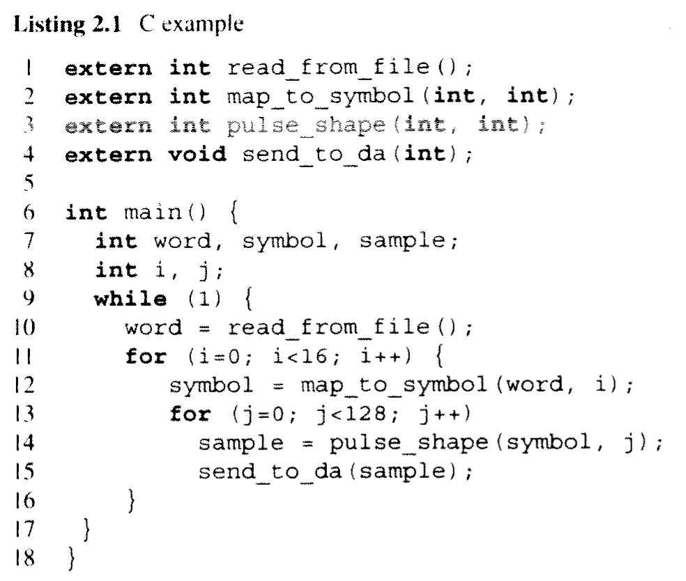
Traditional sequential code does not explicitly support representation of concurrency – difficult to identify opportunities for parallelism when examining the order of operations in the specific implementation
Sequential C Code [†]
Representation of Algorithms
Fig 2.1 Example: Pulse Amplitude System †
The previous diagram made the flow of data clear but does not fully constrain and specify the oder of operations. For instance map and pulse_shape PERHAPS MAY operate in parallel on different symbols in a pipeline. In order to identify the level of parallelism and clearly identify requirements on orders of operation we need a more complete graph. This will more fully constrain the set of possible solutions suggesting a design path.
Data Flow Modeling and Data Flow Graphs
Fig. 2.2
Actors represent functions operating on the data
Actors are linked by queues
Actors may be annotated with relative input and output symbol rates - For example Map generates 16 samples onto its output queue for every sample it pulls from the input
Actors operate independently, they await sufficient data to operate and then place data into output queues
Use of Actors in DFGs represents
Concurrency
Distributed Behavior (as opposed to centralized controller)
Modularity
Fig 2.3
Concurrency: Actors operate and execute individually. Their internal implementation may be for example
sequential code or hardware
Distributed Behavior: the modeling does not require a centralized controller. (In practice we will likely
synchronize and coordinate the implementations of the actors with a controller but is not required and not part of the model)
Modularity: components for actors may be used to develop a library that can be reused in another application
Analysis: high level analysis can performed on graphs to determine conditions such as deadlocks and possible
level of algorithmic parallelism. With C code, verification is often determined by execution on sample data.
Actors:
Contain the the actual operations of data.
Have bounded behavior – precise start and completion
One such iteration is referred to as the actor firing
Tokens: are the conceptual units that carry information from one actor to the other. Token contain values such as 1,4,5,8 in the example below
Queues: are unidirectional communication links with infinite
capacity
Firing rule: describes the necessary and sufficient conditions for an actor to fire – such as number of token available.
Actors may only observe data presented to them from their input queue, they may not observe the state of the system.
Actor firing occurs when data is available on the actor’s input queue(s) according to a firing rule.
Fig 2.3
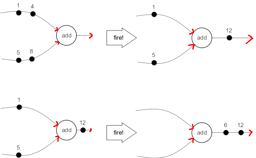
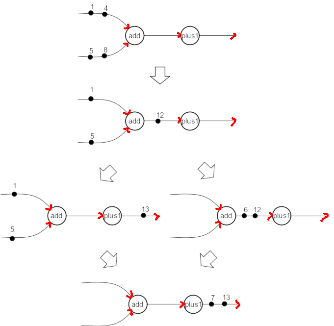
A marking represents a drawn representation of the state of the system and includes a depiction of the tokens present in each queue The evolution of the system involves actors firing. With each firing, actors consume some number of tokens from input queue(s) defined as the token consumption rates and placing tokens on the output queues according to defined production rates
Fig. 2.4 System Evolution depicted by multiple markings
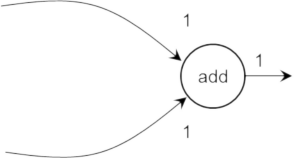
Fig 2.5: Data flow actor with production and consumption rates ꭝ
Example adder with firing rule of one on each input and produces 1 output:
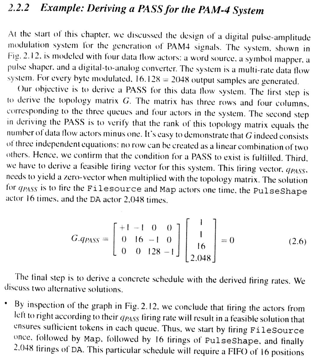
Fig. 2.7 Example of a multi-rate data flow model[ꭝ]
Time is not represented by these models only possible ordering of events and states
Synchronous Data Flow (SDF) Graphs
SDF Graph is a Data Flow Graph for which each actor has a fixed and constant consumption and production rate per fire.
Does not allow for actors to exhibit data-dependent execution (firing based on value of data).
When each actor implements a deterministic function, the SDF Graph is determinate – the output results will always be the same, regardless of firing order.
This means the technology used to implement each actor does not affect correctness of operation.
Fig. 2.8 multiple execution paths to same result †
Deadlocks and Bounded Buffer Links
†
Wish to ensure that a system has valid firing patterns that allow continued unbounded execution without the need for unbounded buffers (infinite capacity queues).
* This precludes a system that requires unbounded storage and systems that reach deadlocks (marking where no actor can fire) under normal input.
SDF Graphs allow testing for these condition by analysis without the need for simulation with data
Periodic Admissible Sequential Schedules (PASS)
A PASS is defined as follows:
A schedule is the order in which the actors must fire
An admissible schedule is a firing order that will not cause deadlock and that yields bounded storage
Finally, a periodic admissible schedule is a schedule that is suitable for unbounded execution because it is periodic. The execution over one period may repeat forever.
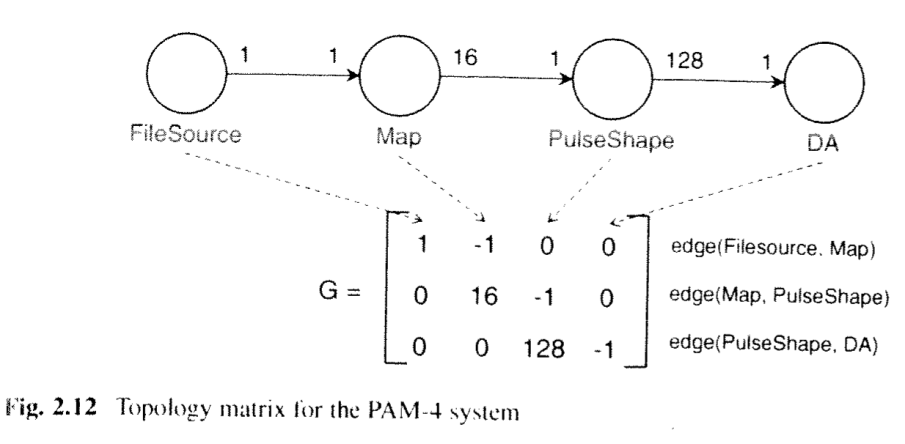
Step 1: Create the topology matrix G of the SDF graph;
Step 2: Verify the rank of the matrix to he one less than the number of nodes in the graph;
Step 3: Determine a firing vector;
Step 4: Try firing each actor in a round robin fashion, until it reaches the firing count as specified in the tiring vector.
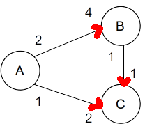
Step 1. Create a topology matrix for this graph. This topology matrix has as many rows as graph edges (FIFO queues) and as many columns as graph nodes. The entry i, j) of this matrix wil be positive if the node j produces tokens into graph edge i. The entry (i) will be negative if the node j consumes tokens from graph edge i. For the above graph, we thus can create the following topology matrix. Note that G does not have to be square -- it depends on the amount of queues and actors in the system.
(2.1)
Step 2. The condition for a PASS to exist is that the rank of G has to be one less than the number of nodes in the graph. The proof of this theorem is beyond the scope of this book, but can be consulted in (Lee and Messerschmitt 1987). The rank of a matrix is the number of independent equations in G. It can be verified that there are only two independent equations in G. For example, multiply the first column with with -2 and the second column with -1, and add those two together to find the third column. Since there are three nodes in the graph and the rank of G is 2, a PASS is possible.
Step 2 verifies that the tokens cannot accumulate on any of the edges of the graph. We can find the resulting number of tokens by choosing a firing vector and making a matrix multiplication. For example, assume that A fires two times, and B and C each fire zero times. This yields the following firing vector:
The residual tokens left on the edges after these firings are two tokens on edge(A,B) and a token on edge(A,C):
(2.2) (2.3)
* Correction Shown: Equation 2.3 Should have solution: [4 2 0] not [2 1 0]
Step 3: Determine a periodic firing vector. The firing vector indicated above is not a good choice to obtain a PASS: each time this firing vector executes, it adds three tokens to the system. Instead, we are interested in firing vectors that leave no additional tokens on queues. In other words, the result must equal the zero-vector. (2.4)
Since the rank of G is less than the number of nodes. This system has an infinite number of solutions, Intuitively, this is what we should expect. Assume a firing vector (a,b,c) would be a solution that can yield a PASS. Then also (2a,2b,2c) will be a solution, and so is (3a,3b,3c). and so on. You just need to find the simplest one. One possible solution that yields a PASS is to fire A twice, and B and C each once: (2.5)
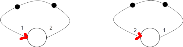
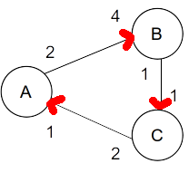
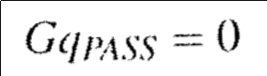
The existence of a PASS firing vector does not guarantee that a PASS will also exist. For example, just by changing the direction of the (A,C) edge, you would still find the same qPASS, but the resulting graph is deadlocked since all nodes are waiting for each other. Therefore, there is still a fourth step: construction of a valid PASS.
Step 4: Construct a PASS. We now try to fire each node up to the number of times: specified in qPASS. Each node which has the adequate number of tokens on its input queues will fire when tried. If we find that we can fire no more nodes, and the firing count of each node is less than the number specified in qpass. the resulting graph is deadlocked.
We apply this on the original graph and using the firing vector (A = 2,B = 1,C = 1). First we try to fire A, which leaves two tokens on (A,B) and one on (A,C), Next, we try to fire B -- which has insufficient tokens to fire. We also try to fire C but again have insufficient tokens. This completes our first round through -- A has fired already one time. In the second round, we can fire A again (since it has fired less than two times), followed by B and C, At the end of the second round, all nodes have reached the firing count specified in the PASS firing vector. and the algorithm completes. The PASS we are looking for is (A,A,B,C).
The same algorithm, when applied to the deadlocked graph in Fig. 2.11, will immediately abort after the first iteration, because no node was able to fire.
Note that the determinate property of SDF graphs implies that we can try to fire actors in any order of our choosing. So. instead of trying the order (A,B,C) we can also try (B.C.A). In some SDF graphs (but not in the one discussed above, this may lead to additional PASS solutions.
Data Flow Limitations
SDF Graphs are Lacking in the modeling following:
Stop and Starting – SDF Model just continuously runs
Mode Switching - structure is fixed at runtime
Exceptions – for instance, “no reset” to globally remove all tokens
Run Time Conditions changing of nodes or condition execution is not allowed (making IF-THEN-ELSE difficult)
Conditional Execution/Firing
Approaches to modeling conditional execution/firing are discussed in the text, including an approach of extending the data flow model.
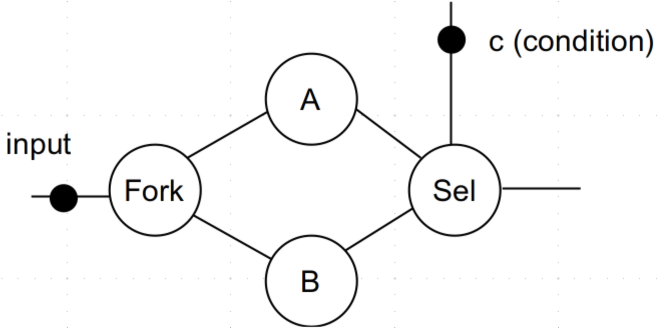
Modeling of IF statements directly using SDF Graphs can be done is as follows
Assumes actors A,B and operate independently on the same data and the actor Sel consumes both results and propagates one or the other
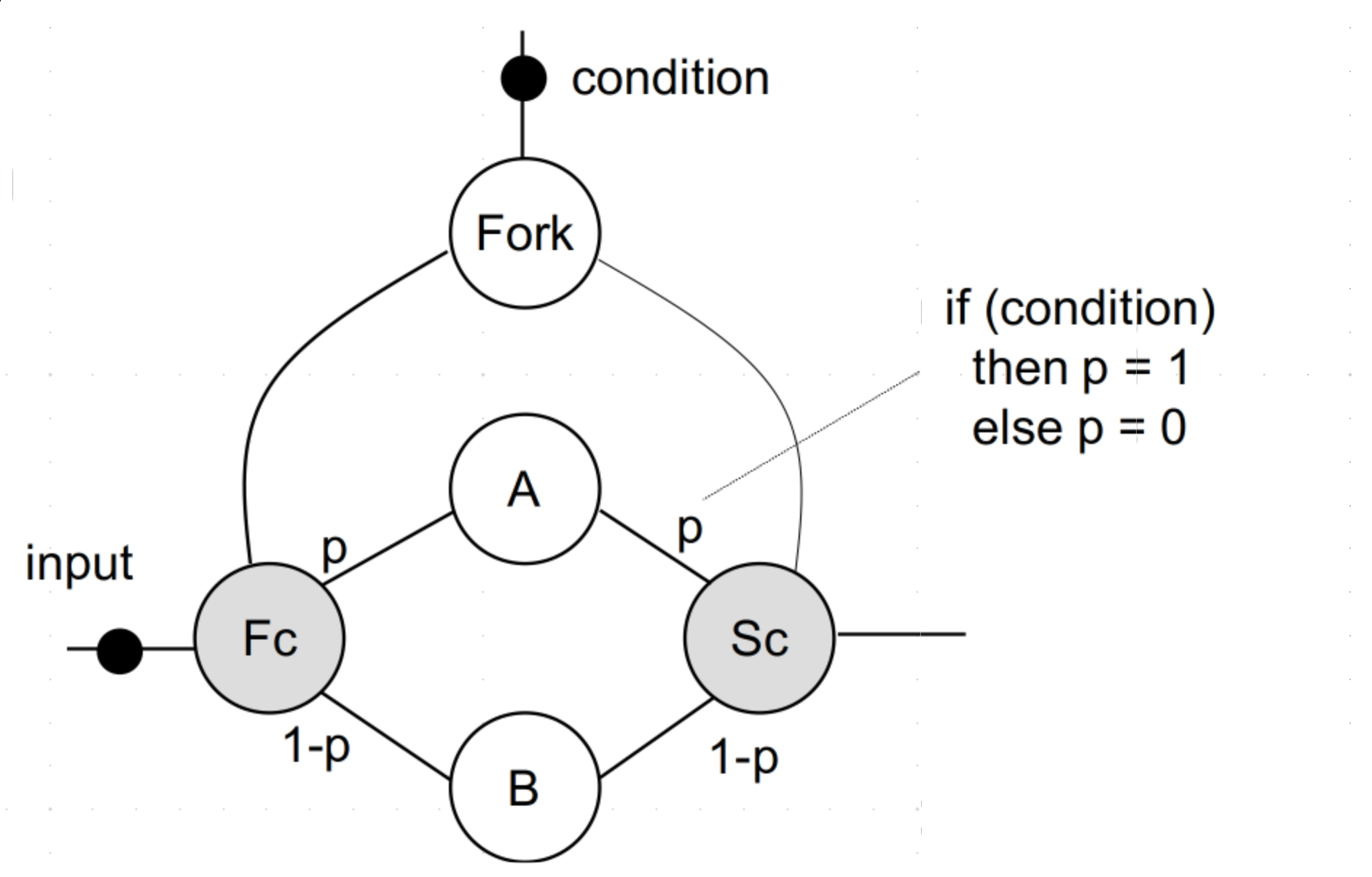
Modeling using extension to SDF
These loose some of the the advantages of SDF. They Involve model under multiple cases and handling of symbolic parameters
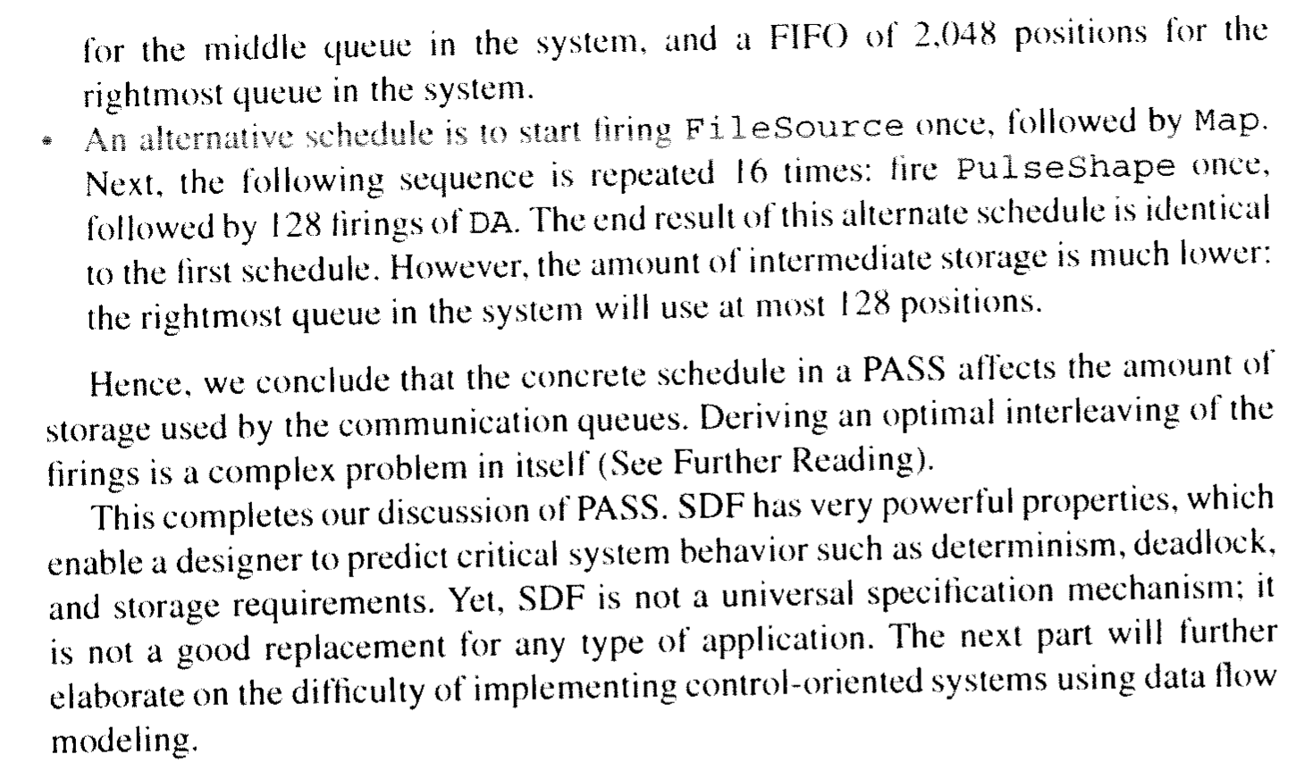
Another Example if time allows: PAM
Time and Resource Modeling
†
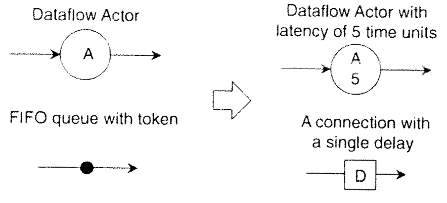
To model the affect of various system transformations we can add minimal resource models.
We can bound queue sizes and introduce latency to actor execution to model throughput.
FIFOs with tokens are instead represented with single-delay units. The number of units along a queue defines the size of the queue
Loop and Iteration Bound
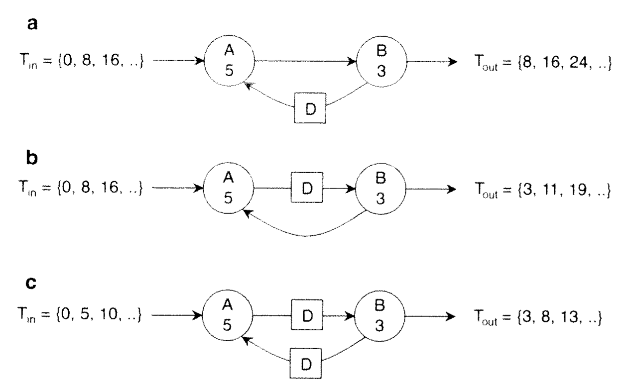
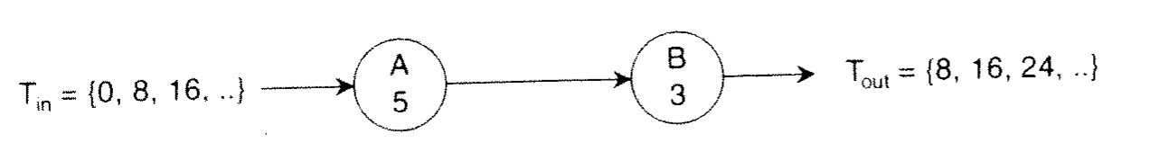
Loop bound – loop execution time/ # delays
Example: Samples per time unit (a) 1/8 (b) 1/8 (c) 1/5 †
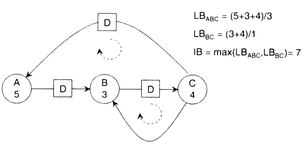
Iteration Bound highest loop bound. It is an upper bound, not necessarily achievable. †
Outer-Loop Loop Bound
†
Loopbound of outer loop or of a linear graph is implied and may also be accounted for
In this case LB = 8

 Printable Version
 []
[]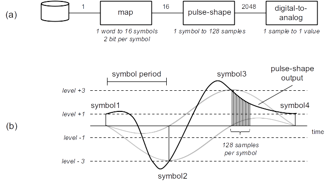
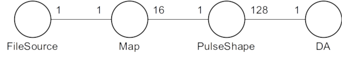 Fig. 2.2
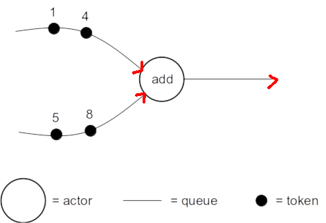 Fig 2.3

 (2.1)
(2.1) (2.2)
(2.2)  (2.3)
(2.3)
 (2.4)
(2.4)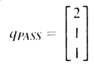 (2.5)
(2.5)