Lecture 06 – Transformations

• Spacebar to advance through slides in order
• Shift-Spacebar to go back
• Arrow keys for navigation

• ESC/O-Key to see slide overview
• ? to see help

Printable Version

Table of Contents

• Lecture 06 – Transformations
  • Table of Contents
  • References
  • Transformations
  • Multirate Expansion
  • Multi Rate Expansion
  • Retiming
  • Pipelining
    • Pipelining with SDF Graphs
  • Piplelining to Meet Timing Requirements
  • Reducing Critical Path of a computation with Pipelining
  • Unfolding (parallelization)
  • Unfolding Recipe
  • Simple Unfolding Example
  • Example 2
  • Unfolding Example 3
  • Unfolding Critical Path and Retiming
  • Unfolding for Low Power
  • Bit-level Parallel Processing

References

• $\dagger$ http://rijndael.ece.vt.edu/gezel2/book.html

• https://en.wikipedia.org/wiki/Unfolding_(DSP_implementation)

Transformations

• Multi-rate Expansion is used to convert a multi-rate synchronous data flow graph into a single-rate synchronous data flow graph.  This transformation is helpful because the the other transformations assume single-rate SDF systems

• Retiming considers the redistribution of delay elements in a data-flow graph, in order to optimize the throughput of the graph.  Retiming does not change the latency or the transient behavior of a data flow graph

• Pipelining is introducing additional delay elements in a data flow graph, with the intent of optimizing the iteration bound of the graph.  Pipelining changes the throughput  and the transient behavior of a data flow graph

• Unfolding increases the computational parallelism in a data flow graph by duplicating actors.  Unfolding does not changes the transient behavior of a data flow graph, but may modify the throughput

Multirate Expansion

• 2.5.1 Multirate Expansion $\dagger$ : It is possible to transform a multi-rate SDF graph systematically to a single-rate SDF graph. The following steps to convert a multi-rate graph to a single-rate graph.
  • Step 1. Determine the PASS firing rates of each actor
  • Step 2. Duplicate each actor the number of times indicated by its firing rate. For example, given an actor A with a firing rate of 2, we create AO and A1. These actors are two identical copies of the same genetic actor A.
  • Step 3. Convert each multi-rate actor input/output to multiple single-rate input/outputs. For example. if an actor input has a consumption rate of 3, we replace it with three single-rate inputs.
  • Step 4. Re-introduce the queues in the dataflow system to connect all actors. Since we are building a PASS system, the total number of actor inputs will be equal to the total number of actor outputs.
  • Step 5. Reintroduce the initial tokens in the system, distributing them sequentially over the single-rate queues (according to the consumers).

Multi Rate Expansion

-based on book figure, colored tokens $\dagger$

• Consider the example of a multirate SDF graph in Fig. 2.19. Actor A produces tokens per firing, actor B consumes two tokens per firing. The resulting firing rates are 2 and 3, respectively.

• After completing steps 1-5 discussed above, we obtain the SDF graph shown in Fig. 2.20. However another adjustment is needed to account for the initial tokens:

• The correction would be to adjust the source of edges a,b,c,d,f according to the number of initial tokens on the original queue (since the initial tokens provide the initial values for those queues). In this example, the first destination without an initial token now receives the first output:

• The actors have duplicated according to their firing rates, and all multi-rate ports were converted to single-rate ports. The initial tokens are redistributed over the queues connecting instances of A and B. The distribution of tokens follows the sequence of B.

• You can verify which one is correct via example, by defining a behavior for the actors. If you consider Figure 2.20, let actor A simply create three copies the input and let actor B add two tokens and produce the sum you can see that it is not correct. From Figure 2.19 if you have an input sequence 1,2,3,.. the output would be 0+0,1+1,1+2,2+2,3+3,3+4,... however in Figure 2.20 the output would be 0+0,1+2,2+2,1+1,3+4,4+4,3+3

• Mult-rate expansion is a convenient technique to generate a specification in which every actor in the system fires at the same rate. For example, in a hardware implementation of data flow graphs, multirate expansion will enable all actors to run from the same clock signal.

• Finally: Step 6. After completing steps 1-5 discussed above, we obtain the SDF graph shown in Fig. 2.20 in the book/lecture notes. Each node is duplicated $R_i$ times according to the firing rate $R_i$ of actor with index $i$. However, another adjustment is needed to account for the initial tokens: adjust the input source of each generated queue according to the number of initial token on the original queue.

  • For each original queue $Q_i$ with $T_i$ initial tokens, let $g_i$ be the number of generated queues labeled $G_0$ to $G_{g_i-1}$. Then the adjustment is the following: in one step shift the source of each generated queue $G_n$ to the pre-shift source of $G_{n-\left(T_i\%g_i\right)}$.

Retiming

2.5.2 Retiming $\dagger$

• retiming is a transformation on data flow graphs that redistributes delays resulting in a "retimed" graph
• retiming doesn’t change the total number of delays between input and output of a data flow graph,
• retiming may increase system throughput
• perform successive retiming transformations, evaluate the performance of each, and choose the optimal

†Shaumont

• Wikipedia:

The initial formulation of the retiming problem as described by Leiserson and Saxe is as follows. Given a directed graph G:=(V,E) whose verties represent logic gates or combinational delay elements in a ciruit assume there is a directed edge e := (u,v) between two elements that are connected directly or through one or more registers. Let the "weight" of each edge w(e) be the number of registers present along edge e in the initial circuit. Let d(v) be the propagation delay through vertex v. The goal in retiming sto compute an integer "lag" value r(v) for each vertex such that the retimed weight $w_r(e) := w(e) +r(v) - r(u)$ of every edge is non-negative. There is a proof that this preserves the output functionality. [C. E, Leiserson, J.B. Saxe, "Retiming Synchronous Circuitry, "Algorithmica, Vol. 6, No. 1, pp. 5-35, 1991.]

†Shaumont

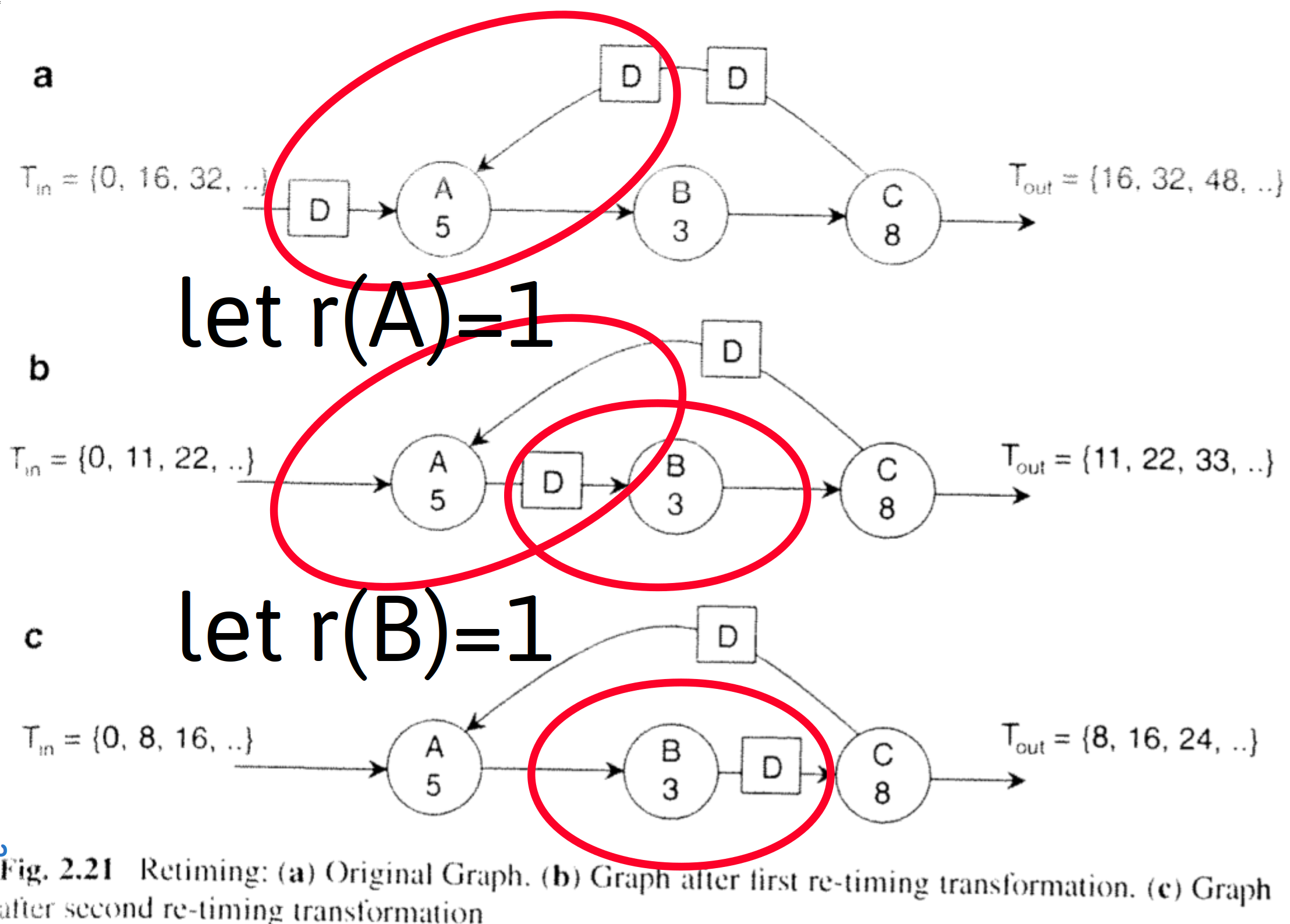
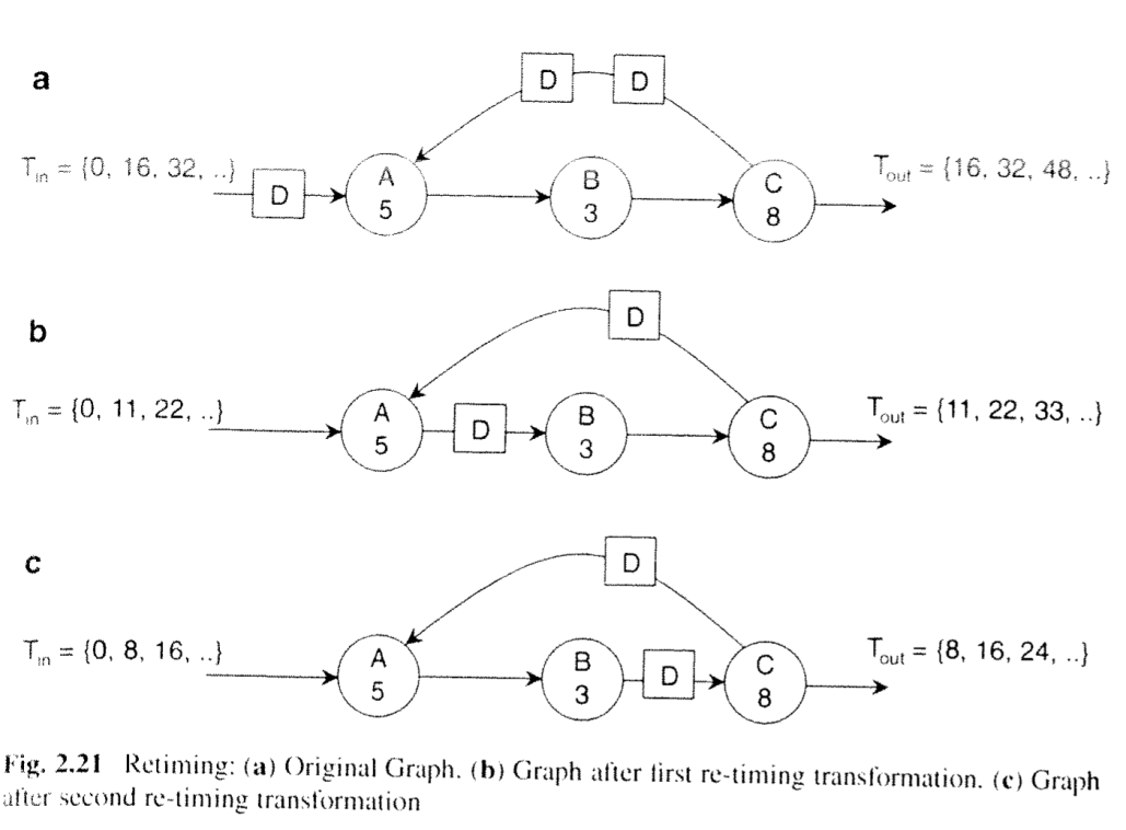
Figure 2.21 illustrates retiming using an example. The top data flow graph, Fig.2.21a, illustrates the initial system, This graph has an iteration bound of 8. However the actual data output period of Fig. 22a is 16 time units, because actors A,B, and C need to execute as a sequence. If we imagine actor A to fire once, then it will consume the tokens (delays) at its inputs, and produce an output token. The resulting graph is shown in Fig. 2.21. This time, the data output period has reduced 11 time units. The reason is that actor A and the chain of actors B and C, can each operate in parallel. The graph of Fig. 2.21b is functionally identical to the graph of Fig. 2.21a: it will produce the same identical stream of output samples when given the same stream of input samples. Finally, Fig. 2.21e shows the result of moving the delay across actor B to obtain yet another equivalent marking. This implementation is faster than the previous one: as a matter of fact, this implementation achieves the iteration bound of 8 time units per sample. No faster implementation exists for the given graph and the given set of actors.

Shifting the delay on the edge BC further would result in a delay on the outputs of actor C: one on the output queue, and one in the feedback loop. This final transformation illustrates an important property of retiming: it's not possible to increase the number of delays ina loop by means of retiming.

Pipelining

Pipelining:

• is the combination of the introduction of added cycle delays followed by retiming

• increases throughput at the cost of increased latency

• The critical path (the slowest pipeline stage in HW) bounds the throughput of the overall system. Retiming efforts, sometimes aided by the introduction of delays, should seek to minimize the critical page.

• Insertion of equal number of tokens/delays at all inputs followed by retiming.

Pipelining with SDF Graphs

by Example Figure 2.22

• Fig.2.22a
  • the critical path (slowest pipeline stage) determines the cycle period, for a system using this subgraph the path is 20 time units at best
• Fig.2.22b is augmented with two pipeline delays producing Fig. 2.22b
  • the critical path determines the cycle period, here it remains as 20 time units
  • System latency increases from 20 to 60 with a THREE-cycle delay of 20 time units each
  • Throughput is 1 sample per 20 time units
• Fig. 2.22b retimed produces Fig. 2.22c
  • the critical path is now characterized by 10 time units
  • The latency is three cycles (number of cycle delays from input to output)
  • The throughput is 1 sample per 10 time units

†Shaumont

Question asked in class: What was the purpose of the second pipeline insertion vs only one here. For example, if C was annotated with 3, would the second pipeline be more justifiable?

Piplelining to Meet Timing Requirements

Critical Path Timing Requirement:
$\rm{T_{CLK-to-Q} + T_{PD} + T_{setup} < T_{clk}}$
Q: What to do if timing requirement is not satisfied?

module calc(q, a, b, c,d clk);
  output q;
  input a, b,c,d;
  input clk;
  reg [31:0] q
  always @(posedge clk) begin: bx
    reg [31:0] tmp1;
    reg [31:0] tmp2;
    tmp1=a*b;
    tmp2=a*b;
    q<=tmp1*tmp2;
  end
endmodule

• Can reduce the clock speed
  • But this slows the entire system
• Can introduce pipelining
  • Overall propagation of computation is longer (two clock cycles incurring multiple setup and hold times)
  • Maintains fast system clock
• Alternatively, may be able to introduce pipelining in the critical path of a system in order to increase the clock rate and therefore overall system throughput

Pipeline

module calc(q, a, b, c,d clk);
  output q;
  input a, b,c,d;
  input clk;
  reg [31:0] q
  always @(posedge clk) begin: bx
    reg [31:0] tmp1;
    reg [31:0] tmp2;
    tmp1<=a*b; //pipeline
    tmp2<=a*b; //pipeline
    q<=tmp1*tmp2;
  end
endmodule

Reducing Critical Path of a computation with Pipelining

Example:
Reducing the critical Path in a moving average calculation:
$$\rm{out}[n]=c_2 \times x[n-2] + c_1 \times x[n-1] + c_0 \times x[n]$$

†Shaumont

†Shaumont

Fig. 2.24 $\dagger$

†Shaumont

Fig. 2.25 $\dagger$

†Shaumont

Fig. 2.26 $\dagger$

Unfolding (parallelization)

• Assume a DSP system computing $$y[n]=a y[n-9]+x[n]$$
• Computing Even and Odd Results (with indexes 2k and 2k+1 respectively where k is any integer) in parallel requires computing $$y[2k]=a y[2k-9]+x[2k]$$ $$y[2k+1]=a y[2k-8]+x[2k+1]$$

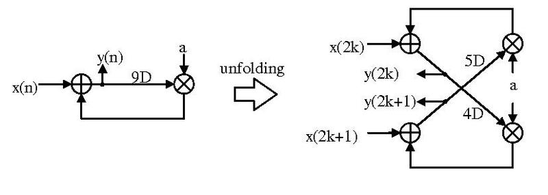
https://en.wikipedia.org/wiki/Unfolding\_(DSP\_implementation)
Image Source: https://en.wikipedia.org/wiki/File:DSP_Folding_example.pdf
Author Jackyknight https://creativecommons.org/licenses/by-sa/3.0/deed.en

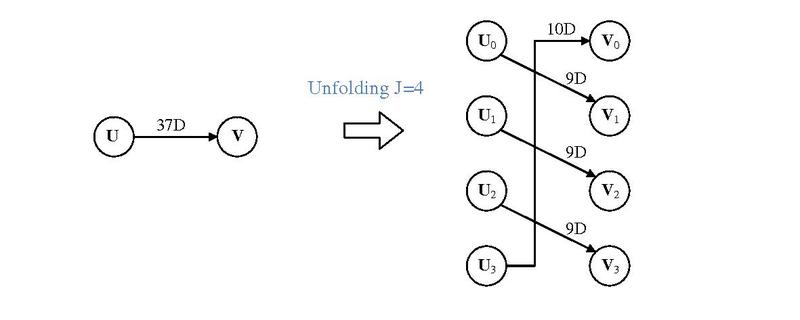
Unfolding Recipe

Sources: Wikipedia and http://www.eecs.yorku.ca/course_archive/2006-07/F/4210/Ch5_unfolding.pdf

To perform $\bm J$-level unfolding:

• Step 1. $\bm J$-replicate nodes ($\bm J$ nodes to replace 1 node): Each node $\bm U$ becomes $\bm U_0 ... \bm U_{j-1}$
• Step 2. Identify edges with delay w going from some node U to another node
  • Let the ${\bm v}$ be the edge $\bm U \rightarrow \bm V$ in the orginal graph to account for
  • In the new graph, ${\rm FOR}\ {\bm i} = 0\ {\rm to}\ {\bm J}-1$, draw new delay edge: ${\bm U}_i \rightarrow {\bm V}_{(i+w)\%{\bm J}}$ with delay $D={\rm floor}\left(\frac{\bm i+\bm w}{\bm J}\right)$
• Step 3. Duplicate inputs nodes $\bm J$ times and label ${\bm A}_0$ to ${\bm A}_{{\bm J}-1}$ each input node ${\bm A}_i$ gets input sequence $x[{\bm J}\cdot k+{\bm i}]$ where k is the sequence 0,1,2,...
• Step 4. If ${\bm J}>{\bm w}$, an edge with delay $\bm w$ in the original graph will result in $\bm w$ edges with delay 1 and ${\bm J}-{\bm w}$ edges with zero delay

Simple Unfolding Example

https://en.wikipedia.org/wiki/Unfolding\_(DSP\_implementation)
Image Source: https://en.wikipedia.org/wiki/File:Unfolding_algorithm_description.pdf
Author Jackyknight https://creativecommons.org/licenses/by-sa/3.0/deed.en

Example 2

†Shaumont

Unfolding Example 3

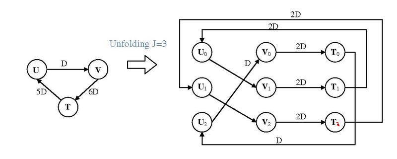
Image Source: https://en.wikipedia.org/wiki/File:Example_of_unfolding.pdf
Author Jackyknight https://creativecommons.org/licenses/by-sa/3.0/deed.en

Unfolding Critical Path and Retiming

• Unfolding has a problem: it may introduce longer critical path.
• New critical paths might be introduced because of new zero-delay edges
  • Assume an $J$-unfolding of an edge with delay $w$, where $w<J$
  • Result is $w$ paths have delay one, and the remaining $J-w$ have no delay
  • These new zero-delay edges can form a new critical path in the system
• Pipelining and Retiming may be used to compensate after unfolding

Unfolding for Low Power

• Duplicating the hardware by a factor N and reducing the speed by a factor of N can yield lower power assuming a better than linear tradeoff in speed and power (e.g. through use of alternate technologies or alternate modes of operation)

• Unfolding implements Parallel processing, which can be exploited for lower power operation instead of higher throughput
  • Con: The number of components is increased
    ( linearly, by J ) and thus the total capacitance (routing likely increases a bit more since the average routing distances across the components would likely grow)
  • Pro: With parallel processing, circuity can operate lower speeds, this allows lowering the supply voltage
  • Many transistor circuits operate more efficiently (power vs speed) at lower supply voltages. Thus, there is a better than a linear tradeoff in power and speed (e.g. the half-speed implementations are less than half the power, or the system somehow benefits such as through the use of more power-efficient computing devices )
  • Hence parallelization offers the possibility for lower power operation.

Bit-level Parallel Processing

• Example shows a 4-bit bit-serial processor converted to a bit-parallel processor (https://en.wikipedia.org/wiki/Unfolding_(DSP_implementation)

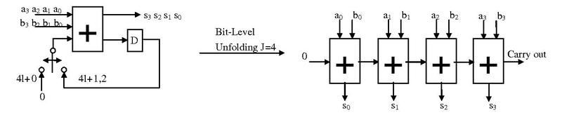
Image Source: https://en.wikipedia.org/wiki/File:Bit-level_unfolding.pdf
Author Jackyknight https://creativecommons.org/licenses/by-sa/3.0/deed.en

• Here, note the reduction of the number of registers and a longer combinatorial data path.
• If this is not the critical path of the system in which it is used, it may be a good trade-off to perform unfolding of this subsystem