Lecture 11 Metastability
Ryan Robucci
1. References
- ꭝ High Speed Digital Design: A Handbook of Black Magic 1st Edition by Howard Johnson (Author), Martin Graham (Author)
2. Digital Abstraction and Noise
- consider a chain of digital gates
- signal corruption model: ideal gates with noise sources
- desire proper interpretation of binary values in presence of noise
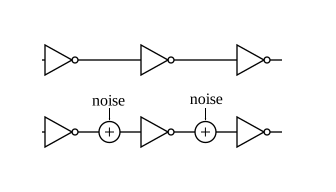
- Sources of Noise:
- 1) Electronic Thermal Noise
- 2) Power/Ground Current (through supply resistance)
- 3) Fast Signals in the System (large dI/dt induces drops in supply inductance)
- 4) Signal Coupling: Mutual Cap. and Mutual Inductive
- 5) Ringing (will draw in-class if required)
- 6) Temperature Differences between components affecting threshold voltages
(3-5 are especially important for fast systems)
Additionally, manufacturing between devices can introduced fixed noise, which may be exhibited as device-specific offsets
3. Noise Margins
- Noise margins ensure correct digital operation, maintaining the digital abstraction
- Require voltage constraints on inputs, and outputs to satisfiy input constraints for the downstream gate even in the presence of noise
- The difference between the output and input constraint are known as the **Noise Margin**s
- Noise Margin High is the margin for logical high: \(V_{\rm NNH}=V_{\rm OL}-V_{\rm IH}\)
- Noise Margin Low is the margin for logical low : \(V_{\rm NNL}=V_{\rm IL}-V_{\rm OL}\)
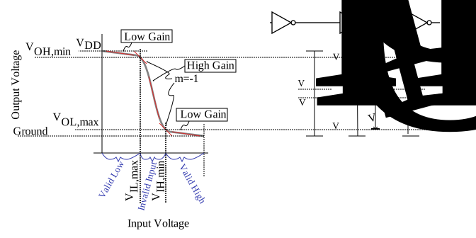
- Digital Gates restore weak values by the low gain in the valid input regions.
- Typical in this context to denote gain of -1 (slope=-1) as boundary of low gain and high gain
- Inputs in the valid regions safely produce valid outputs even when corrupted with noise
- Inputs in the invalid region can produce high or low outputs with moderate noise
4. Noise F.O.M.
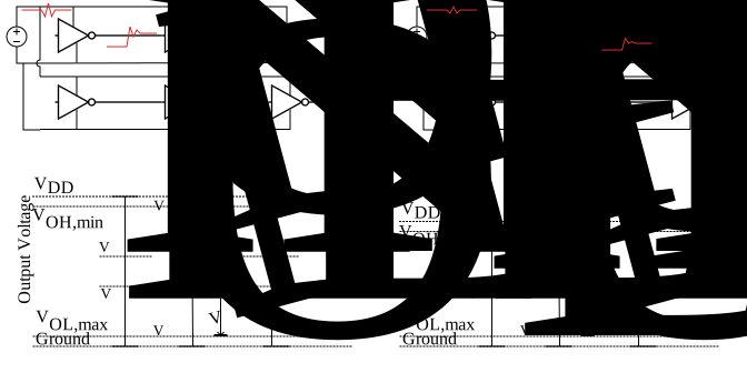
- Some corruption is proportional to voltage swings
- Examples:
- larger transition \(\rightarrow\) larger ringing
- larger transition \(\rightarrow\) larger disturbance on neighboring signal lines
- Examples:
- Noise Performance Figure of Merit: Ratio of Noise Margin to Voltage Swing is a useful figure of merit (FOM)
For example: for two logic families, noise margins that are proportional to the power supply level may perform roughly the same \({\rm FOM} = \frac{\rm Noise\ Margin}{\rm Voltage\ Swing} = \frac{V_{OH}-V_{IH}}{V_{OH}-V_{OL}}\) or \(\frac{V_{IL}-V_{OL}}{V_{OH}-V_{OL}}\)
- for those that like %: magnitude the noise may be quantified as a percentage of full voltage range
5. Timing Requirements for Registers
- Registers tend to have voltage as well as specific timing requirements for the inputs
Setup and Hold

- If violated, may get
- Old Data
- New Data
Metastable Output
- Not conform to voltage specifications
- May change in middle of clock period (multiple output transitions triggered by the clk)
Possible Output transitions when expected is 0->1:

6. Clock Domain Crossing
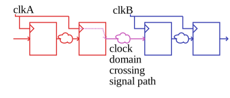
- Clock Domain Crossing arises from the need to communication between Multiple Clock Domains
- You have learned in sync. design in one clock domain
Having Multiple Clock Domains means Clock Domain Crossing must be considered
7. Async Inputs
Not all signals arise from a clock domain at all, such as physical, real-world inputs
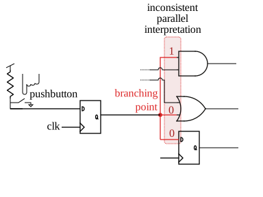
A problem arises at a fanout point, where mutiple interpretations are performed in parallel. If the voltage is not a valid high or valid low, inconsistent interpretations can result.
8. Metastabilty
Consider that an inverter represents contrain on allowed input, output (\(V_1\),\(V_2\)) relationships:


The graph on the right shows how V2 is driven.
Consider another inverter with the input and output connections are exchanged:


The graph on the right shows how V1 is driven.
Consider a coupled set of inverters, setting constraints between V1 and V2


Set of constraints and underlying drive on V1,V2:


Two constraints, A and B Three Points are possible solutions to both constraints 1 is a quasi stable solution

9. Temporal Dynamics Analysis
Time analysis:

Consider ideal voltage sources and switches set two intial voltages Switches are opened at time t=0
Case 1:
\(V_1(0) = 0\) \(V_2(0) = {V_{\rm DD}}\)
\(V_1 \rightarrow 0 \Rightarrow \boxed{\mathcal A} \Rightarrow V2 \rightarrow V_{\rm DD} \Rightarrow \boxed {\mathcal B} \Rightarrow V_1 \rightarrow 0\)
Case 2:
\(V_1(0) = {V_{\rm DD}}/2\) \(V_2(0) = {V_{\rm DD}}/2\)
\(V_1 \rightarrow {V_{\rm DD}}/2 \Rightarrow \boxed{\mathcal A} \Rightarrow V2 \rightarrow {V_{\rm DD}}/2 \Rightarrow \boxed {\mathcal B} \Rightarrow V_1 \rightarrow {V_{\rm DD}}/2\)
Case 3:
\(V_1(0) = \frac{3}{4} {V_{\rm DD}}\) \(V_2(0) = \frac{1}{4} {V_{\rm DD}}\)
\(V_1 \rightarrow \frac{3}{4} {V_{\rm DD}} \Rightarrow \boxed{\mathcal A} \Rightarrow V2 \rightarrow 0 \Rightarrow \boxed {\mathcal B} \Rightarrow V_1 \rightarrow {V_{\rm DD}}\)
\(V_1\) is pushed to VDD, system stabalizes @ (\(V_1\) = VDD, $V2$=0)
Case Quasistable:
In theory, the middle point is also stable We have assumed a symmetric transfer function and constraints


However, any noise will disrupt the balance. If \(V_1\) is bumped more positive, \(V_2\) is pushed more negative and thus \(V_1\) is pushed more positive, etc… Positive Feedback ensure until \(V_1=V_{\rm DD}\) and \(V_2=0\)
10. Quasi-stable
Hill analogy
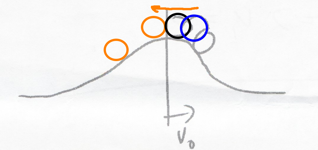
- Think of of the quasi-stable point in the analogy of balancing a ball on a hill:

- Middle point is quasistable and can only be preserved in a noiseless system. Starting points to the left of middle are pushed towards the left and starting points on the right are pushed to the right

Quasi-stable point is only preserved (without external input) in a noiseless system
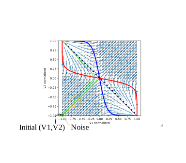
Field and Energy:


Example Trajectories one WITH and the other WITHOUT noise:
11. Types of Memories
First consider for what types of memories this is relevant:
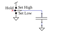
Capacitor-Storage Based
- Capacitor and switch:
- Resistive (e.g. memristor, magnetic storage) or other physical state changes
- Latch (Positive Feedback) Based
SRAM
Two Inverter (SRAM):

S-R Latch:

Clocked (Level Sensitive) SR Latch

Clocked D-Latch:

alternative view as extension of clocked SR latch:

12. Time to Settle

The question of interest is how long does is take to reach a stable state as a function of starting position?
Given \(V_A(0)\) how long to reach a stable point?
Given T, a time limit to reach stable point, what is the constraint on \(V_A(0)\)?
13. Metastabilty Cause
- Clocked latches can be placed near a metastable state if the clock transitions while data is

- The problem is more than complex than "will it settle to the new or old value?" If placed in a metastable state, the output can be stuck near the quasistable point for a very long time and the following stages will non-deterministically interpret the signal as 1 or 0 depending on thresholds and noise
- Latches are vulnerable to corruption when they are in a state near the quasi-stable point
- Transitions disrupted at the wrong time can be delayed reversed, or even undergo multiple transitions
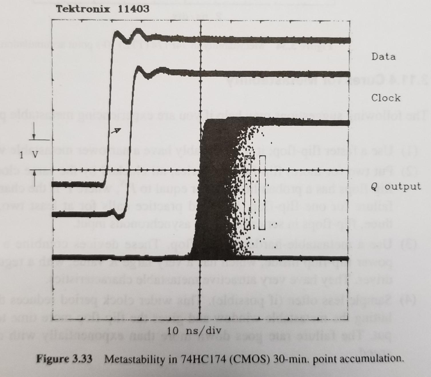
 ꭝJohnson and Graham
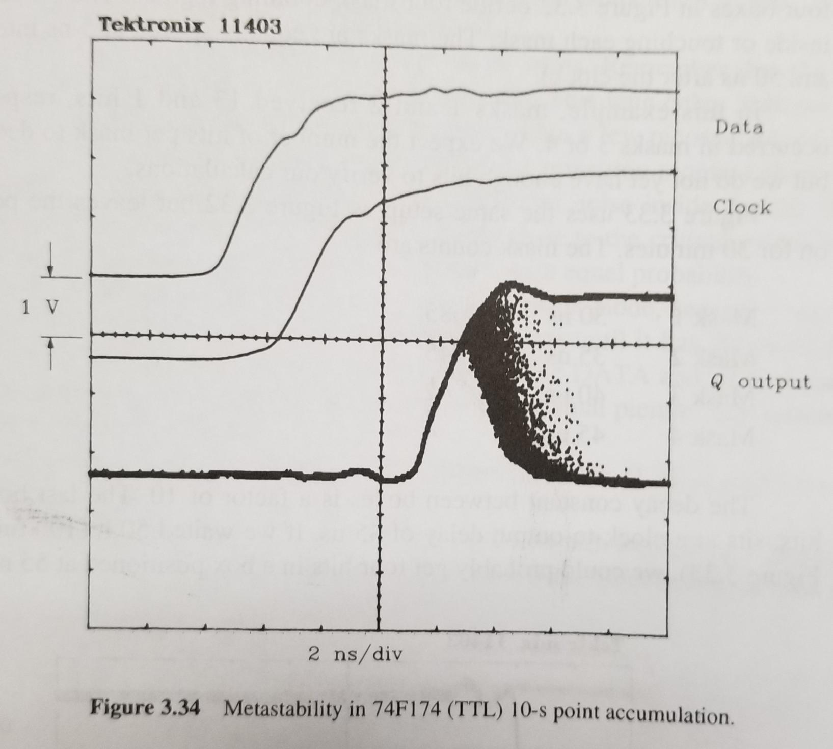
 ꭝJohnson and Graham
 ꭝJohnson and Graham
14. Parallel Resolution of Two Signals
Assume in the Logic, D0 and D1 represent two values that are sampled and sent into an AND gate.
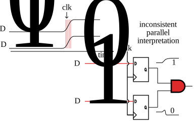
Here the AND output may glitch and become low in error if the inputs change at a disallowed time.
15. Parallel Resolution at Fanout Point
At some point in the system, parallel resolution can cause a problem
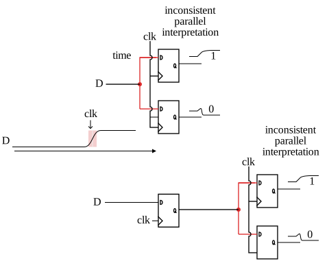
The same input signal (staring point) can be resolved differently in two components

16. Temporal Analysis
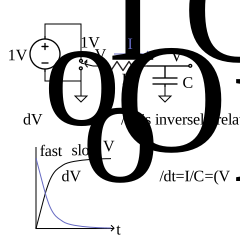
A generic, 1st-order representation of positive feedback:

Assume the Ideal Amp, at all times \(V_B = V_A \cdot A\)
Positive Feedback
- General behavior of positive feedback is to accelerate away from a quasi stable point (VA=VB=0)

- Negative feedback for comparison: fast than slow settle at a equilibrium
Transient Analysis
- Analyze the temporal voltage change at the input storage capacitor. The voltage value here represents the state of the system
\(\frac{dV_A}{dt}=\frac{I}{C}=\frac{V_B-V_A}{R \cdot C}=\frac{A V_A-V_A}{R \cdot C}\)
\(\frac{dV_A}{dt}=\frac{(A-1) V_A}{R \cdot C}\)
\(V_A(t) =V_A(0) e^{t\,\,\underbrace{\frac{A-1}{RC}}_K}\)
The Question:
Time to reach VDD/2 ?
The Answer:
- Approach:
- Solve for \(t\) in \(V_A(t) = V_{DD}/2\)
- \(t=\frac{1}{K} \ln \left(\frac{V_{DD}/2}{V_A(0)} \right)\)
- This is the time to reach \(V_{DD}/2\) given some starting point \(V_A(t=0)\)
17. Time and Voltage Constraint
Bound t to be less than a desired clk-to-Q, i.e. time to resolve, \(T_r\) , and find \(|V_A(0)|_{\rm min}\)
\(T_r = \frac{1}{K} \ln \left(\frac{V_{DD}/2}{V_A(0)}\right)\)
\(V_A(0) = \pm \left(V_{DD}/2\right)^{-1} e^{T_r K}\)
- \(T_r\) and \(V_A(0)\) here represent the time and voltage constraints on the input

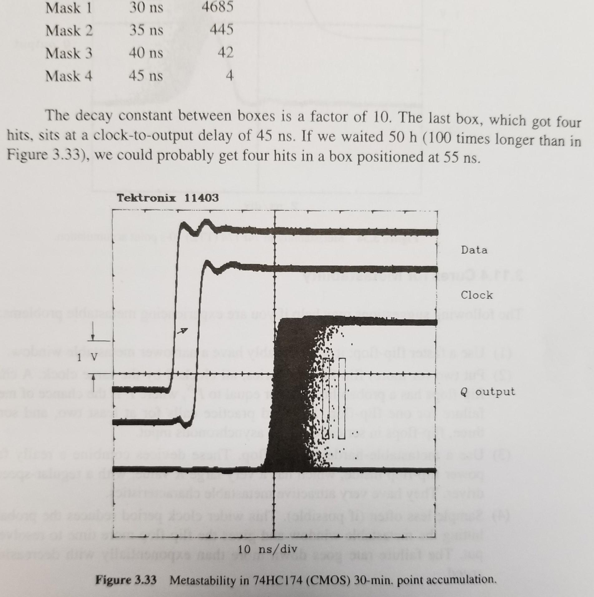
- Starting values farther from the metastable equilibrium than \(|V_A(0)|_{\rm min}\) will resolve quickly
- Starting values closer to the metastable equilibrium than \(|V_A(0)|_{\rm min}\) will resolve in a much longer amount of time, and meanwhile are more susceptible to noise corruption
- Nature of Exponentials (Self-similarity)

- Leads to relationship: linear input voltage -> exponential settling time
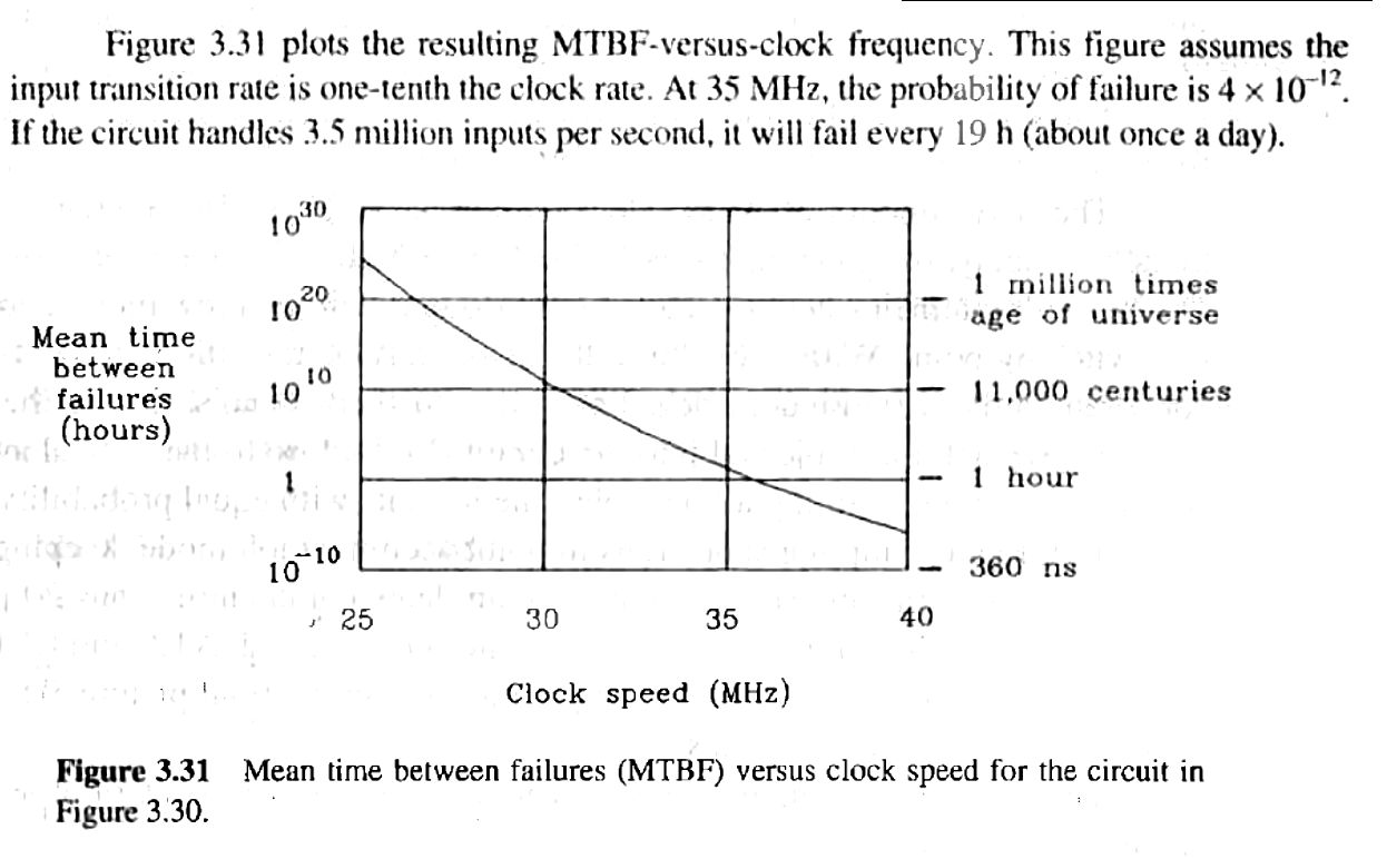
See the mask counts on the next page for 30-min accumulation:
 ꭝJohnson and Graham
18. Implication of Metastabilty
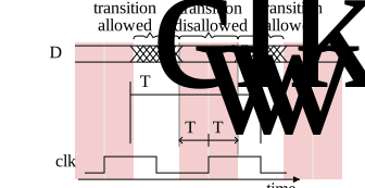
- For a given rise time, an input transition must stay outside a time window around the clock event:

- The implication of data transition slope and timing is that the rise time and allowed arrival time of a 50% transition point are related:

Data as Reference
For the next analysis: instead of viewing the clk as the reference and data timing as the variable

consider the data edge to be the reference

\[2|T_W| \approx \frac{2 V_A(0)}{\frac{V_{\rm DD}}{T_{\rm 10-90}}} \] \[2|T_W| \approx T_{\rm 10-90} e^{-KT_r}\]
- If clock rises in in the data window, the output may not settle in time [eq 3.34]:
\[|T_W| = C e^{-KT_r}\]
- C is a constant (maybe found empirically), rise-time is a primary component
19. System Timing Requirements
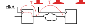
\[\boxed{T_r \lt \frac{1}{F_{\rm clk}} - T_{PD}} \rightarrow T_W=Ce^{-K \boxed{T_r}}\]
\(T_{\rm W}\) defines the window of error [eq 3.36] that helps define setup and hold time requirements and thus allowed combinatorial propagation delays
20. Operation Timeline
- Assume a uniformly random arrival of Data:
- Chance of MS Problem is [3.37]

- Probability of Failure Per Data Transition:
\[ P = \frac{2T_W}{T_{\rm CLK}} = 2F_{CLK}Ce^{-KT_r} \] (this is the likelihood that a random transition falls in a disallowed epoch)
- Assume
- in given time span \(T_{\rm span}\) there are \(N\) data transitions expected
- each transition having probability P of causing a failure,
- The expected # of failures in that timespan
\[N\cdot P \text{ failures in timespan } T_{\rm span}\]
- The rate of failure is the rate of data transitions times the probability of a given transition causing a failure
\[\frac{N}{T_{\rm span}} \cdot P = \rm Expected\,Rate\,of\,Failure\]
21. Mean Time Between Failures
The Rate of Failure is INVERSELY RELATED TO the mean time between failures
\[{\rm MTBF} = \frac{1}{R\cdot P};R=\frac{N}{T_{\rm span}}\] R is the data transition rate
- When looking at various documents and datasheets, you may see many alternative forms but with similar underlying form
Actel 1989 ACT-1 Logic:
- Sample Switch Rise Time Constant \(C = .5\times10^{-9}\)
- Response Time Constant \(K = 4.6052 \times 10^{9}\)
- ꭝPage 127: R (rate of transitions) is 1/10th of the clock rate:
 ꭝJohnson and Graham
22. Mitigating Metastability
1) Faster FF
a faster flip-flop naturally has narrowed metastability window
2) N-FlipFlops in a row:
known as the simplest synchronizer to move into a clock domain or between clock domains
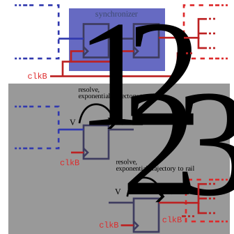
Effective Time provided is doubled (2T):
\(V_3(2T)=\underbrace{V_2(T)}_{V_3(T)}\underbrace{e^{KT}}_{\text{update}}=V_1(0)e^{KT}e^{KT}=V_1(0)e^{K2T}\)
\(T_W=Ce^{-2KT}=C\left(e^{-KT}\right)^2\)
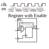
\begin{aligned} {\rm if\,\,} P_{\rm fail} \propto& {T_W} = C\overbrace{e^{...}}^{K_1} {\rm \ \ \ \ \text for\,1\,\,flip-flop} \\ \\ {\rm then}\\ P_{\rm fail} & = {C}{K_1^2} {\rm \ \ \ \text for\,2 \,flip-flops} \\ P_{\rm fail} & = {C}{K_1^N} {\rm \ \ \ \text for\,N\,flip-flops} \end{aligned}Another Possibility to realize this effect for a multi stage (e.g. master-slave) flip-flop that can be implemented with RTL in with only a single register and a single clock domain without a gated clock:
3) Metastability-Hardened FF
rather than just a use higher-power fast FF, it would be a low-power flipflop specifically designed with large K)
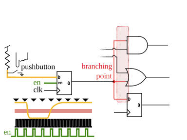
4) Sample Less Often
enable input capture (sample) less frequently, which sacrifices responsiveness
5) Use Edge-Sharpening Amplifiers at the Input
fast input transitions lessen the likelihood that an invalid input is sampled
